APPLIED INDUSTRIAL CONTROL SOLUTIONS
ApICS LLC.
Digital Filter Design
Writing Difference Equations For Digital Filters
Brian T. Boulter
© ApICS ® LLC 2000
ABSTRACT
Difference equations are presented for 1st, 2nd, 3rd, and 4th order low pass and high pass filters, and 2nd, 4th and 6th order band-pass, band-stop and notch filters along with a resonance compensation (RES_COMP) filter. The low pass, high pass, bandpass and bandstop difference equations are obtained from the normalized butterworth continuous time filter descriptions given below.
1st. order normalized Butterworth low pass filter:
 (1.0a) (1.0a)
2nd. order normalized Butterworth low pass filter:
 (1.0b) (1.0b)
3rd. order normalized Butterworth low pass filter:
 (1.0c) (1.0c)
4th. order normalized Butterworth low pass filter:
 (1.0d) (1.0d)
2nd. order normalized Notch filter
 1.1a) 1.1a)
4th order normalized Notch filter
 (1.1b) (1.1b)
6th. order normalized Notch filter
 (1.1c) (1.1c)
Normalized Res_Comp filter
 (1.1d) (1.1d)
The above low pass filter (not the notch or RES_COMP filters) equations are mapped to the appropriate filter type using the following mappings.
To map (1.0x) to a lowpass filter use:
 ; ;  = desired low-pass 3 [d.b.] cutt-off frequency. (1.2) = desired low-pass 3 [d.b.] cutt-off frequency. (1.2)
To map (1.0x) to a highpass filter use:
 ; ;  = desired high-pass 3 [d.b.] pass frequency. (1.3) = desired high-pass 3 [d.b.] pass frequency. (1.3)
To map (1.0x) to a bandpass filter use:
 (1.4) (1.4)
where:
B = A number that controls the bandpass depth/width (equivelant to 1/Q).
 = The desired continuous time center frequency. = The desired continuous time center frequency.
To Map (1.0x) to a band-stop filter use:
 (1.5) (1.5)
where:
B = A number that controls the notch depth/width (equivelant to 1/Q).
 = The desired continuous time center frequency. = The desired continuous time center frequency.
For example if we want to obtain a fourth order band-stop filter we use equation (1.0d) and use the mapping of equation (1.5) after some algebra we obtain the following continuous filter description:

To create a digital filter we normalize the above filter by setting  = 1, and map to the z-domain using the bi-linear transformation: = 1, and map to the z-domain using the bi-linear transformation:
 (1.6) (1.6)
The c co-efficient in the above equation is used to accomplish frequency warping. That is, to compensate for an inherent inaccuracy in the bi-linear transformation method that is a function of frequency and sample rate. (see any D.S.P. text for a more complete explanation)
Once the above mapping is performed by substituting (1.6) into the continuous time s-domain filter equation we obtain a z-domain transfer function of the form:
 (1.7) (1.7)
Where, for any filters obtained using the normalized low-pass butterworth filter as the basis for the digital filter, n = d = order of the filter. For low-pass to low-pass and low-pass to high-pass mapping the order of the digital filter is the same as the order of the starting normalized butterworth filter. For low-pass to band-pass and low-pass to band-stop mapping the order of the digital filter is twice the order of the starting normalized butterwoth low-pass filter.
Let:
 the normalized notch center frequency. (i.e. the normalized notch center frequency. (i.e. 1) 1)
 = the desired notch center frequency = the desired notch center frequency
 = Sample time in sec. = Sample time in sec.
The warping equation is given as:
 (1.8a) (1.8a)
The RES_COMP filter which uses the same mapping as above, requires that the
denominator resonant frequency be post-warped with (1.8b) below.
 (1.8b) (1.8b)
After some algebra we obtain the following co-efficients in (1.7) for low-pass, high-pass,
band-pass and band-stop filters for the indicated order of the filter.
Low-Pass Filter
n=1

n=2

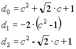
n=3

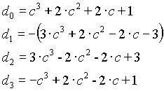
n=4


High-Pass Filter
n=1

n=2

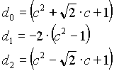
n=3

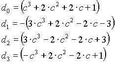
n=4

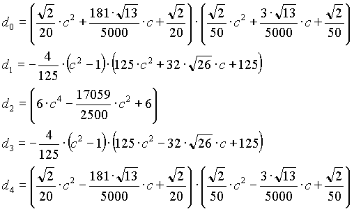
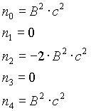
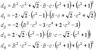
Band-pass filter
n=2


n=4
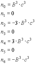
n=6

Note:
1) B in the above equations is equavelant to 1/Q; where Q is the depth factor in notch filter
designs.
Band-stop filter
n=2


n=4
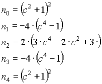

n=6
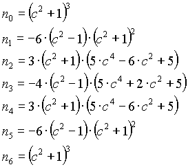

Note:
1) B in the above equations is equavelant to 1/Q; where Q is the depth factor in notch filter
designs.
Notch filter
n=2
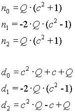
n=4
Proprietary
n=6
Proprietary
RES_COMP filter
Proprietary
Notes:
1)  is the zero compensation frequency with damping equal to is the zero compensation frequency with damping equal to  /2. /2.
2)  is the pole compensation frequency with damping equal to is the pole compensation frequency with damping equal to  /2. /2.
CREATING THE DIFFERENCE EQUATIONS:
From the z-domain transfer function we obtain the difference equation as follows:
Know from (1.7)
 (1.9) (1.9)
Therefore (1.9) becomes

In difference equation form:

or in terms of the latest output:
 (1.10) (1.10)
Where for each filter described above the appropriate co-efficients are used in (1.10).
|